✿ code toolkit ✿ python ✿

✿ Review from last week ✿

Variables

A variable is a placeholder for a value

New syntax:

creatureX = 50
rect( creatureX, 100, 20, 50 )

New vocabulary:

You create a variable by assigning it a value, as in the first line above. (Unlike in many other programming languages, in Python you do not need to declare a variable before using it.)

Then you can use that variable throughout your code. You can use basic arithmetic to modify it's value. For example using:

+ — addition
- — subtraction
* — multiplication
/ — division

And you can even make one variable depend on the value of others. For example:

creature1X = 100
creature2X = 500
midpoint = ( creature1X + creature2X ) / 2
# What would the value of midpoint be now?

Anytime you want something in your code to change (or "vary") you need to add one or more variables.

We thought a bit about how many variables you would need to represent a given composition, and this can be a useful first step in project planning.

Question: If you wanted to draw 3 creatures and you want them to move around on the screen horizontally and vertically, how many variables would you need?

Answer: You would need 6 variables: one for the x and y values of each creature.

And if you then also wanted the height of each creature to change? You would need three more.

Interaction Discussion

So far we have been working with Processing in what is known as static mode. We've been creating sketches that draw some shapes and then end.

Today we are going to introduce dynamic movement and respond to user input in what Processing refers to as interactive mode.

Let's think about ways of representing movement, motion, and gestures.

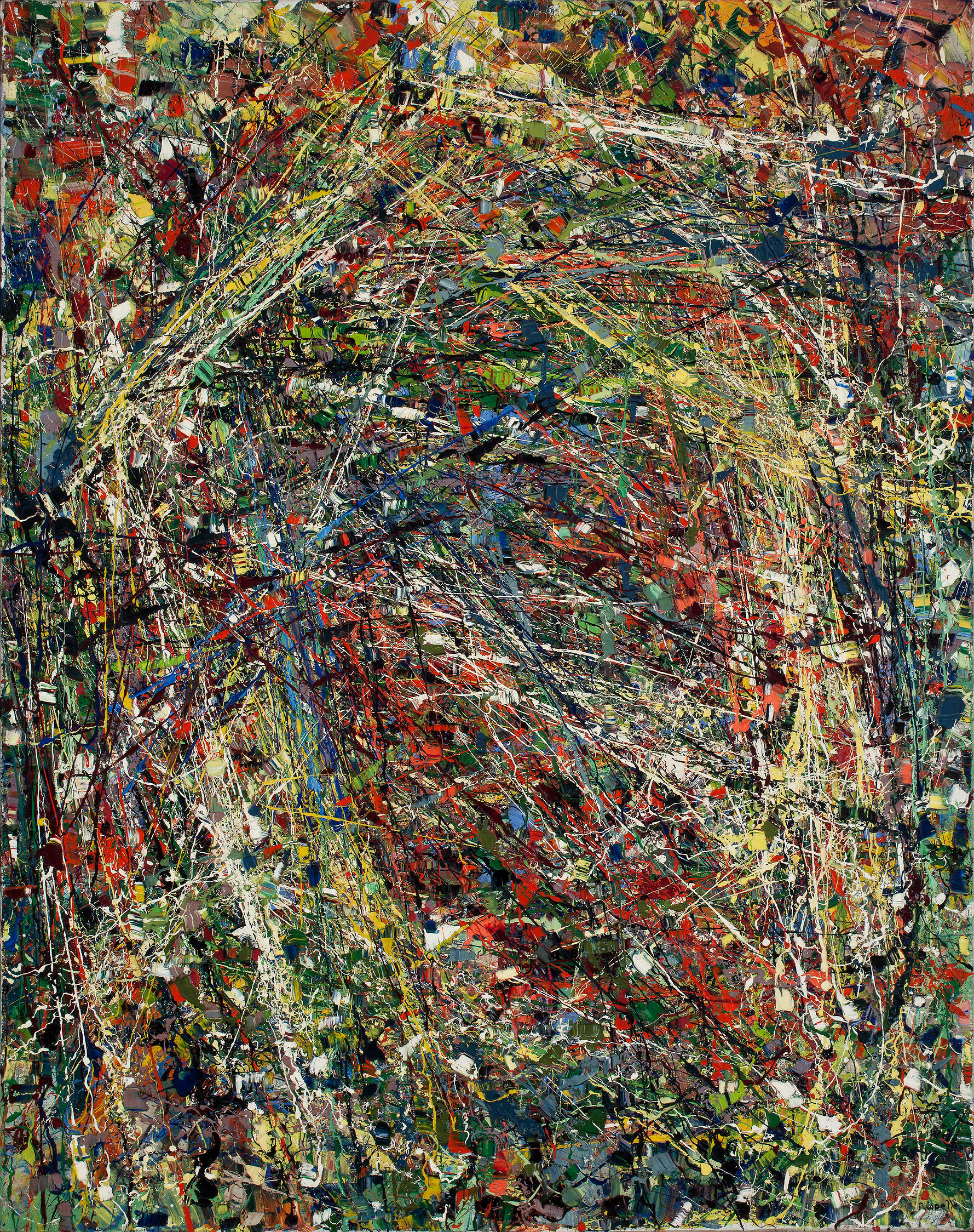
Below is an image from Jean Paul Riopelle, an abstract expressionist painter. The period in which Abstract Expressionism was popular occured just after WWII. AE was understood to be using color and shape to create visual compositions that were often wholly abstract, not representations of any actual objects in the world, and were often interpreted as being highly expressive, depicting only feelings, energy, mood, or affect.

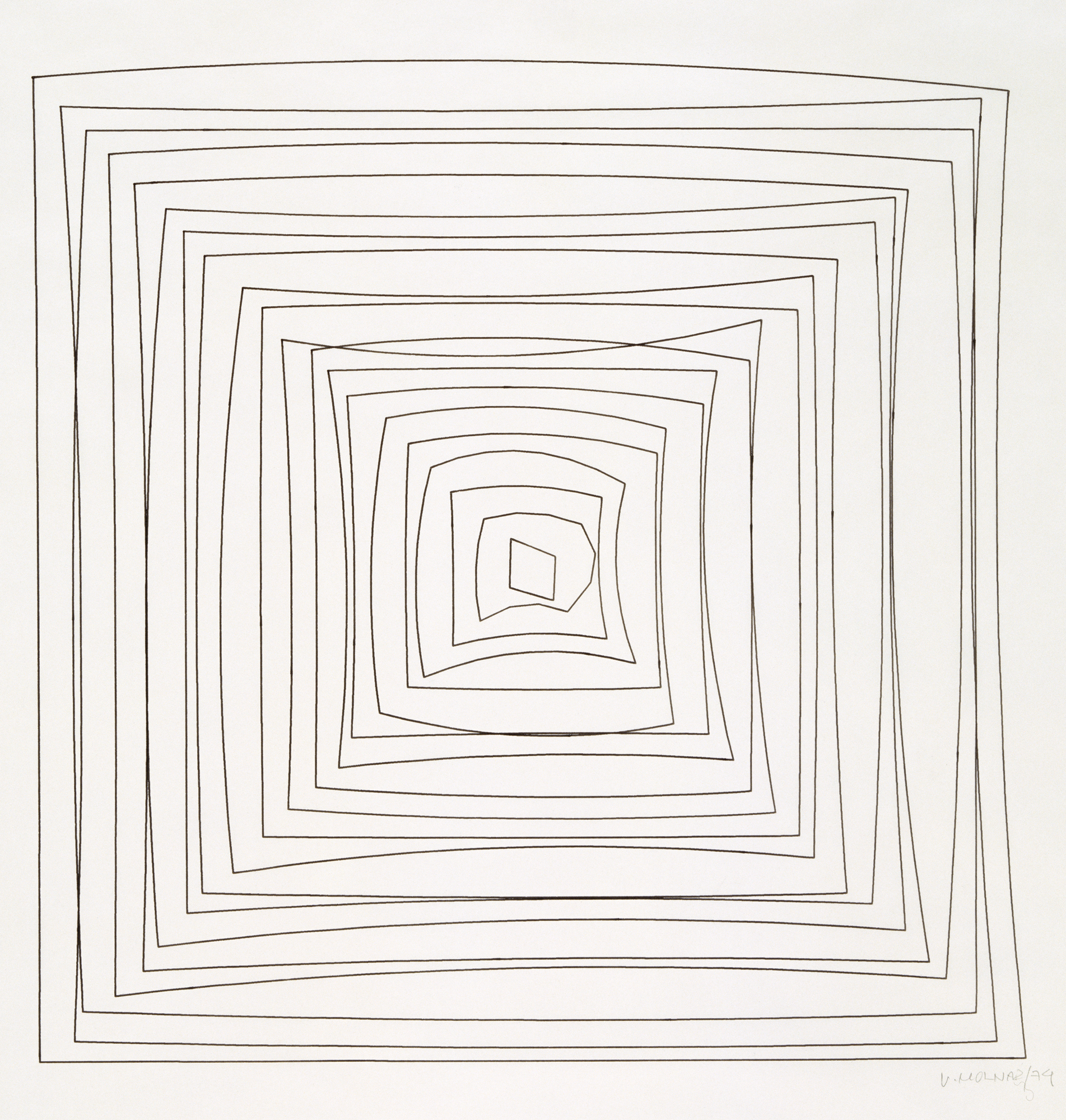
Taking up some of the main themes in abstract expressionism, computer art pioneer Vera Molnar prioritized chance and the mistake in her work. This allowed for her works to have a kind of motion and gesture akin to motion and gesture you might find in early abstract expressionist work.

In an interview with Hans Ulrich Obrist, he asks Vera: what is the role of randomness in your work? Is randomness at the heart of what you do? Or not? And she replies:

Listen, if you replace the word ‘random’ with ‘intuition’, there you have it. With intuition, suddenly you say – now what if I used a curve instead of a straight line and what sort of a curve? And then you try it – that’s intuition. Randomness does the same thing.

For this week, as we begin to learn about using code to respond to user input, let's keep in mind this idea of creating compositions that capture or represent movement and motion, and do so in a way that aim to be expressive of mood, affect, or feeling of the person creating them.

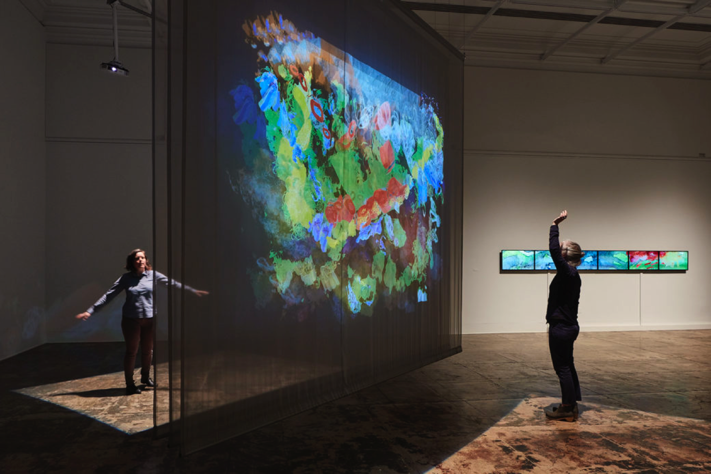
There is much precedent within digital art for thinking about these kinds of representations. Artists like Camille Utterback, Golan Levin, Zach Lieberman, and others, have created work in a genre often referred to as interactive art. (And we can think of what Lev Manovich's "myth of interactivity" here: that human-computer interaction is always already interactive and so using the word to describe work in this genre is tautological.) But these kinds of "interactive" works rely on user input, in the form of movement, gesture, or play, is often necessary to enact or complete the piece.

Utterback's pieces, for example, use the movement and actions of viewers to generated colorful expressive compositions full of wide arrays of texture and form. They use sophisticated computer vision techniques to sense user motion via the motion of bodies standing in front of a large screen. For this week we will focus only on mouse movement. But towards the end of the semester there will be the opportuntity to play with more advanced computer vision techniques.

Golan Levin's project Yellowtail (1998-2010) is another great example. This project was originally created before Processing existed, but then was re-written for Processing in 2007. At one time it was easy to run in a web browser, but due to various technology and business decisions, most browsers no longer support Java applets, and so it probably won't run for most of you. Levin has made it available as an iOS app for 99¢. You can watch some video documentation of the project here.

Bringing together these threads (interactive art, abstract expressionism) is a fun project simply called "Jackson Pollock" by designer Miltos Manetas: jacksonpollock.org. (In order to run it you may need to download the .swf file and double click on it.)

✿ Adding interactivity with Processing ✿

Processing comes with certain pre-defined variables. For example width and height, which will always reference the width and height of the draw window, no matter what.

Another special variable is mouseX which tracks the x position of the mouse.

Let's try to create a sketch that draws a rectangle whose x position is the x position of the mouse. Our initial attempt might be something like this:

size(400,400)
background(255)
stroke(50,50,255)
fill(200,200,255)
rect(mouseX,150,100,100)

But that doesn't work. Why not?

This is using Processing's static mode. That means that this code runs once and then stops. In the language of digital media, we might say that it creates one single frame. But in order to create movement, we need to create many frames in sequence. That code draws a rectangle at the initial value of mouseX, which happens to be 0, and then it never draws another frame, so even as the mouse moves (and the variable mouseX is updated) the sketch never has the chance to redraw the rectangle.

In other words, it's almost like that sketch creates a photograph. Remember this is all we we're doing in our first assignment. What we want to do now is create a movie: multiple photographs that go by in sequence.

In Processing, we do this with some new syntax:

def setup():
    # This block of code runs once

def draw():
    # This block of code runs many times

You can use this in Processing in the following way:

# Create your variables here

def setup(): 
# Initializing code that you want to run once goes here 

def draw():
# All drawing code goes here

But now you have to pay close attention to indentation: the amount of spaces at the start of each line. Last week I told you that Python and Processing don't care about whitespace (spaces, newlines, tabs) and this is mostly true. But one situation in which Python requires you to be very precise about whitespace is with indentation.

The term for these new code structures introduced here is a code block, or just block. A block is a chunk of code that gets run together in some way. We will look at several other types of code blocks in the coming weeks, but right now we're just looking at the setup() and draw() blocks.

In Python, you indicate the start of a new block with a colon (:), and then you indicate all the code in that block by indenting it with the same number of spaces. The block continues on every line until you stop indenting. We will be using 4 spaces. (You are allowed to use different numbers of spaces or tabs, as long as you are consistent. Programmers love to fight over which is the best to use. This semester we will use 4 spaces for consistency and later on you can do whatever you'd like!)

Let's demonstrate this with the following example:

def setup():
    println("Doing this once.")  

def draw():
    println("Doing this many times.")

If you run this code and look in the Processing Console, you will see some interesting output. Press the Stop button (so that you are able to scroll back) and scroll back to the top of the Console. Notice that the code inside setup() does happen only once, and the code inside draw() happens many times.

This code introduces a new command: println(). Usually pronounced as "print line", this command prints arbitrary text in the debugging window at the bottom of the PDE. You write this text as characters in double quotes “ ”, which are called strings. The most famous example of this in introductory programming is the well known "Hello, world!" example:

println("Hello, world!")

In addition to strings, we can also print variables:

x = 5
println(x)

This can be extremely useful for debugging later on when you are trying to figure out what the value of a variable is.

And we can combine words and variables using the plus sign (+). When the arguments to + are strings, it does not do arithmetic, but instead does string concatenation, just mashing together the text of the string with the value of the variable. Having one operator that can be used for more than one purpose is called operator overloading, and it can be very confusing, but it can also be a convenient shortcut. We'll try not to use too many other examples of operator overloading this semester.

But if you try to run this example:

x = 5
println("x is now equal to " + x)

You will get an error. Processing is telling you exactly what and where the problem is. You can fix it by using the str() command.

x = 5
println("x is now equal to " + str(x))

Frame

This idea of doing things many times introduces a new concept called a frame. Similar to a single frame in a movie, a single frame in Processing (as well as in most digital media) is one single static image. Like in a movie or stop-motion animation, flipping through many static images in sequence gives the impression of movement.

How many times per second does it run? Processing provides a special variable to tell you this called frameRate. You can use println() to examine the value of this variable:

def draw():
    println(frameRate)

As you can see, the frame rate is slightly changing all the time! This is because the actual frame rate (the number of times per second that Processing is able to run the draw() block) depends on things like how fast the computer's processor is, how many other programs are running, etc. For reference, the frame rate of most cinema is 24 frames per second (or "fps").

In Processing, you can adjust this with:

frameRate(24) # 24 is now the number of frames per second

Note that the parameter here indicates the maximum frame rate. Processing may not be able to acheive that frame rate (due to processor speed, etc.) but that is what it will try to do.

Returning to the original example, we can merge together the code that tries to draw a rectangle using mouseX with the above setup() and draw() code:

def setup():
    size(400,400)

def draw():
    background(255)
    stroke(50,50,255)
    fill(200,200,255)
    rect(mouseX,150,100,100)

We should always put size() inside setup() because we only need to do that once, and we put all the other draw code inside draw() so that it will happen many times per second. Now each time that Processing runs the draw(), the special variable mouseX will contain the current location of the mouse and the rectangle will be drawn there.

Scope

Using the setup() and draw() code blocks like this introduces a new concept called scope. This important term describes the parts of your sketch in which different variables are accessible. The following code gives an error message:

def setup():
    i = 0

def draw():
    rect(i,0,50,50)

Why? Because the scope of i is limited to setup(), or in other words, the variable can only be used inside setup(), meaning within the chunk of code that is indented together after the colon following setup(). In the above example, i is being used inside draw(), but the variable is not accessible there.

So another way of describing this would be: since the variable i is defined inside the setup() block, its scope is limited to that block and it is not accessible from within the draw() block.

To fix this error, you can move your declaration of i into global scope, in other words, outside of all indented code blocks. In that way, your variable will be accessible in all blocks. Like this:

i = 25
def setup():
    size(100,100)

def draw():
    rect(i,0,50,50)

This is called a global variable. People usually don't like global variables. They can create code that is very confusing to read. But in Processing they are required.

Confusingly, whenever you assign a variable a value within a block, Python tries to create a new variable within that block. So for example, look what happens when you run this code:

i = 0
def setup():
    size(100,100)
    i = 25	

def draw():
    rect(i,0,50,50)

You might think the rectangle would get drawn with x at 25, but it gets drawn with x at 0. Why? Because i = 25 inside setup() creates a new variable limited to that scope. The solution is the global keyword. Whenever you want to use a variable in more than one scope, you must declare it to be global within the various code blocks where you will use it. So modify the above code like this:

i = 0
def setup():
    size(100,100)
    global i
    i = 25	

def draw():
    rect(i,0,50,50)

and now it will do the expected thing.

To simplify: you should create your variables in global block (this is just at the very top of your code, no indentation), and then declare them as global inside each block where you want to use them.

When?

Now that we have introduced the concept of frames into our sketches, and our programs unfold in time, it begs an imporant question. In regards to a command or code instruction, we can now ask: When does that happen? Before today, this question didn't really matter. Over the last two weeks, the only sense of time that mattered was the order in which your instructions were run — from top to bottom, which created visual objects from back to front — but all that happened in a split second and didn't really matter in terms of "human" time. But now the sketch has a duration that we humans can perceive, and things can happen over time. So, when?

The original example of this lesson draws a rectangle at the x location of the mouse:

def setup():
    size(400,400)

def draw():
    background(255)
    stroke(50,50,255)
    fill(200,200,255)
    rect(mouseX,150,100,100)

But look what happens if we move background() out of draw() and into setup():

def setup():
    size(400,400)
    background(255)

def draw():
    stroke(50,50,255)
    fill(200,200,255)
    rect(mouseX,150,100,100)

Running this now leaves a trail of rectangles from all previous mouse positions. Why? Because background() only runs once, only wiping the screen at the beginning of the program, but Processing runs the draw() block many times per second, each time creating a frame, and without background(), Processing draws new rectangles without erasing the previous ones. Depending on your intention, there are times when you may or may not want this effect.

As another example, think about how this relates to random(). You used this command to set variables to random values. But now whenever you use random() you must ask yourself an important question when is the random command being called? When is that random number being chosen? Consider this example:

def setup():
    size(400,400)
    background(255)
    r = random(0,255)
    g = random(0,255)
    b = random(0,255)
    fill(r,g,b)

def draw():
    rect(150,150,100,100)

Each time you stop and run that sketch, the rectangle will have a different color. Three random values are chosen inside setup() and the fill color is set once at the beginning of the sketch.

Now let's make a slight change:

def setup():
    size(400,400)
    background(255)

def draw():
    r = random(0,255)
    g = random(0,255)
    b = random(0,255)
    fill(r,g,b)
    rect(150,150,100,100)

We have moved the selection of random values and the setting of the fill color into draw(), meaning that new random values are selected and the fill color is set each frame. This creates a very different effect.

Again, there are different times that you may want each of these different behaviors.

Interaction, continued

So far we've talked about the special Processing variables mouseX and mouseY. We saw that as the mouse moves, Processing automatically sets the value of these variables to the x and y position of the mouse in every frame.

There are several other special variables that Processing provides us, and now I want to talk about two more:

pmouseX, and pmouseY.

Every frame, Processing sets the values of these variables to the x and y position that the mouse was at on the previous frame. This can be very useful for achieving some interesting effects.

Let's look at the line() command.

This draws a line (a direct path between two points) to the screen.

Syntax
line(x1, y1, x2, y2)
Parameters
x1 float: x-coordinate of the first point
y1 float: y-coordinate of the first point
x2 float: x-coordinate of the second point
y2 float: y-coordinate of the second point

Putting these two things together, let's try to draw a line from the location of the mouse in the previous frame to the location of the mouse in the current frame:

def setup():
    size(400, 400)
    strokeWeight(10)
    stroke(155,155,255,50)

def draw():
    background(255)
    line(pmouseX, pmouseY, mouseX, mouseY)

You might see a little something there, but not much. Why? Because the frame rate is so fast that as the user moves the mouse, even quickly, there is still only a small distance between the location of the mouse on the previous frame and the location of the mouse on the current frame. Let's lower the frame rate to make this a little easier to see:

def setup():
    size(400, 400)
    strokeWeight(10)
    stroke(155,155,255,50)
    frameRate(4)

def draw():
    background(255)
    line(pmouseX, pmouseY, mouseX, mouseY)

Now that there are only four frames per second, we can move the mouse quickly and better see the relationship between the location of the mouse in the previous frame and the location of the mouse in the current frame.

There is a lot that can be done with this principle. Let's use the distance between the previous and current mouse positions to do something besides draw a line, like specify the width and height of a shape.

Simply by subtracting the previous mouse position from the current mouse position, we are calculating the distance that the mouse moved between these two frames.

Writing that up in code form:

def setup():
    size(400, 400)
    noStroke()
    fill(155, 155, 255, 50)
    frameRate(4)

def draw():
    background(255)
    ellipse(200, 200, mouseX-pmouseX, mouseY-pmouseY)

Distance is difference

Distance is calculated by subtracting. (What about negative values? Fortunately Processing handles that for us in this case, but ideally we should do an absolute value here to make sure we only have positive values. The need for this will be eliminated when we use dist() below.)

Now let's run that and see what happens. We are using the distance as the width and height of the ellipse. Try moving the mouse horizontally, vertivally, and diagonally to see how the width and height are affected. As you can see, distance is also related to speed. The faster the mouse is moved, the more distance it covers between frames.

Now what if we want to do something a little more complicated with distance? What if we wanted to set the thickness of a line based on how fast the user is moving the mouse. So, the faster the movement (the more distance between frames), the thicker the line.

As many of you have already experimented with, line thickness is specified with strokeWeight(), and as you can see from the Processing reference, this takes one parameter, which corresponds to the thickness of the line in pixels. Our distance calculation above produced two values (distance in x and distance in y). How can we get just one value? Simple subtraction was enough for determining distance in x and in y separately, but to actually determine the distance between any two arbitrary points requires some more complicated geometry calculations.

Anyone remember how to calculate the distance of this line? (Hint: your old friend Pythagoras ...)

Fortunately, we don't have to worry about that because Processing offers us a shortcut for doing this calculation: dist().

As you can see from the reference, dist() takes four parameters: the x and y values of one point, and the x and y values of another. And it automatically calculates the distance (in pixels) between them.

So how would we calculate the distance between the mouse position of the previous frame and the mouse position of the current frame?

dist(pmouseX,pmouseY, mouseX,mouseY)

Putting that into a complete sketch:

def setup():
    size(400, 400)
    stroke(155, 155, 255, 50)
    frameRate(4)

def draw():
    background(255)

    d = dist(pmouseX,pmouseY, mouseX,mouseY)
    strokeWeight(d)

    line(pmouseX,pmouseY, mouseX,mouseY)

There are some issues with this. For one, the line gets really thick really quickly! Also, what if we wanted to create something that felt kind of like a pen or a brush, in the sense that the line got thinner as the user moved faster, and thicker as the user moved slower. Fixing these two issues leads us to the next topic ...

Map

To address the above questions, let's look at map(). This is a simple thing that can be very useful, but it can be a little tricky to understand.

map() takes a variable and translates (or "maps") it from one range of values proportionally into another range of values. It will be very useful to anyone who elects to do a data visualization for their midterm project.

map()takes a number, in some range, and translates ("maps") that proportionally into some other range.

As the reference explains, it takes four parameters:

map(value, low1, high1, low2, high2)

It assumes that value is between low1 and high1, and then it translates that into the range of low2 and high2.

It might be best to start by illustrating this with some examples:

map( 5, 0,10, 0,100 ) # Answer: 50

map( 5, 0,10, 50,100 ) # Answer: 75

map( 5, 0,10, 60,70 ) # Answer: 65

map( 3, 0,4, 0,100 ) # Answer: 75

You can also go from high to low, instead of low to high:
map( 3, 0,4, 100,0 ) # Answer: 25

Here are some practical examples that you can re-use in your code:

If you wanted a rectangle to move up/down in the same direction as the mouse, but limit it to a region smaller than the full window, you could do this:

rectY = map(mouseY, 0,height, 100,200)
rect( 200,rectY, 50,50 )

If you wanted a rectangle to move left/right in the opposite direction as the mouse, you could do this:

rectX = map(mouseX, 0,width, width,0)
rect( rectX,200, 50,50 )

If you wanted to create a fill color controlled by the mouse x that was always shades of red, you could do this:

r = map(mouseX, 0,width, 0,255)
fill(r,0,0)

The following sketch illustrates some things that you can do with this command:

def setup():
    size(400, 400)  
  
def draw():
    background(255)

    strokeWeight(1)
    stroke(0)
    noFill()
    rect( 5, 150, 10,100)
  
    strokeWeight(10)
    stroke( 55, 55, 255)
    line( 10, mouseY-10, 10, mouseY+10)

    strokeWeight(1)
    fill(155, 155, 255, 150)

    y1 = map( mouseY, 0, height, 150, 250)
    rect( 200, y1, 50,50)
  
    y2 = map( mouseY, 0,height, 250,150)
    ellipse( 250, y2, 50,50)

    x1 = map( mouseY, 150, 250, 200,width)
    triangle( x1,350, x1,375, x1+25,375)

    size1 = map( mouseY, 150, 250, 25,200)
    ellipse( 50, 350, size1,size1)
  
    amt = map( mouseY, 150, 250, 0,1)
    c1 = color(255,55,55,100)
    c2 = color(55,255,55,100)
    c = lerpColor( c1, c2, amt)
    fill(c)
    noStroke()
  
    ellipse(300,100,75,75)
    ellipse(350,110,30,30)
    ellipse(300,50,30,30)
    ellipse(350,75,50,50)
    ellipse(275,50,20,20)
 

Returning the original example that motivated this, how could we make a line that behaves somewhat like a pen or a brush, in that the line gets thinner as the user moved faster, and thicker as the user moved slower. We can use pmouseX and pmouseY along with map():

def setup():
    size(600, 600)
    stroke(155, 155, 255, 50)
    background(255)

def draw():

    distance = dist(pmouseX, pmouseY, mouseX, mouseY)

    mappedDistance = map(distance, 0,200, 40,1)
    strokeWeight( max(mappedDistance,2) ) # using max() to set a maximum value here

    line(pmouseX, pmouseY, mouseX, mouseY)

Another application of this is to create a parallax effect using map() with raster images:

"""
 Inspired by:
      http://1morecastle.com/wp-content/uploads/2013/01/parallax-scrolling-mario.gif

 The images referenced below are available here:
   - http://composingdigitalmedia.org/ccr/week03-mountains.png
   - http://composingdigitalmedia.org/ccr/week03-hills.png
   - http://composingdigitalmedia.org/ccr/week03-foreground.png
 Download these and save them into your sketch folder.
"""

def setup():
    size(800,375)

    global mountainsImage
    global hillsImage
    global foregroundImage

    mountainsImage = loadImage("week03-mountains.png")
    hillsImage = loadImage("week03-hills.png")
    foregroundImage = loadImage("week03-foreground.png")

def draw():

  rg = map(mouseX, 0,width, 155,10)
  b = map(mouseX, 0,width, 255,50)
  background(rg,rg,b)

  mtnX = map(mouseX, 0,width, 0,-20 );
  image(mountainsImage, mtnX,50)

  hillsX = map(mouseX, 0,width, -20,-200 )
  image(hillsImage, hillsX,250)

  fgX = map(mouseX, 0,width, 0,-2000 )
  image(foregroundImage, fgX,225)

  darkness = map(mouseX, 0,width, 0,225)
  fill(0,darkness)
  rect(0,0,width,height)

That sketch uses three images. You can download them here:

Mountains Hills Foreground